DSMC-Neutrals Case Study - Pumping to High Vacuum Simulation
DSMC-Neutrals is a 3D rarefied gas analysis software package that utilizes the Direct Simulation Monte Carlo (DSMC) method. By employing an unstructured mesh, it enables simulations of complex geometries. It also supports chemical reaction calculations, making it suitable not only for simulating rarefied gas flows within vacuum chambers but also for modeling thin-film deposition in semiconductor manufacturing processes such as Chemical Vapor Deposition (CVD). If reading this article has made you even slightly interested in rarefied gas analysis or gas flow simulation, please feel free to contact us at any time to request materials or for further information.
Introduction
Since DSMC-Neutrals uses an unstructured mesh, it is capable of simulating equipment with complex geometries.
For example, this allows us to evaluate the conductance of piping connected to a turbo molecular pump.
In this session, we will use a simplified model to evaluate the conductance of piping and orifices as well as the pumping curve (evacuation time) inside the vacuum chamber.
Furthermore, by comparing these results with theoretically derived conductance values and pumping curves, we hope you will appreciate the practical value of performing these simulations.
Conductance and Pumping Time of Short Pipe
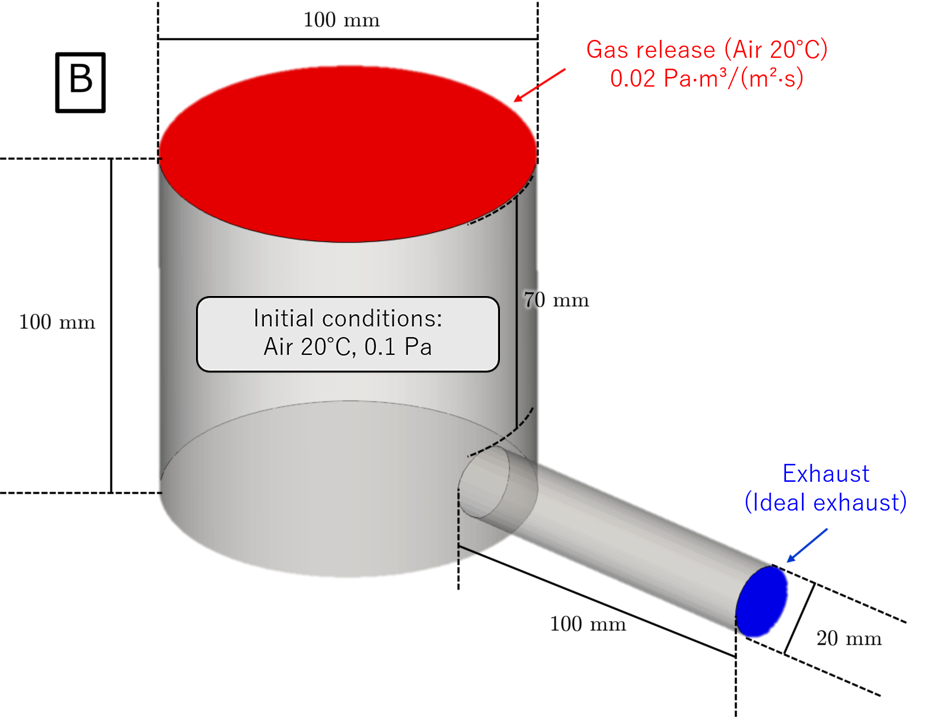
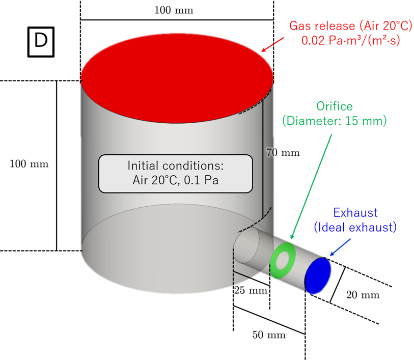
First, we will consider the simulation model shown below as the standard model for this case study. (For convenience, we will refer to this model as "standard" or "A".)
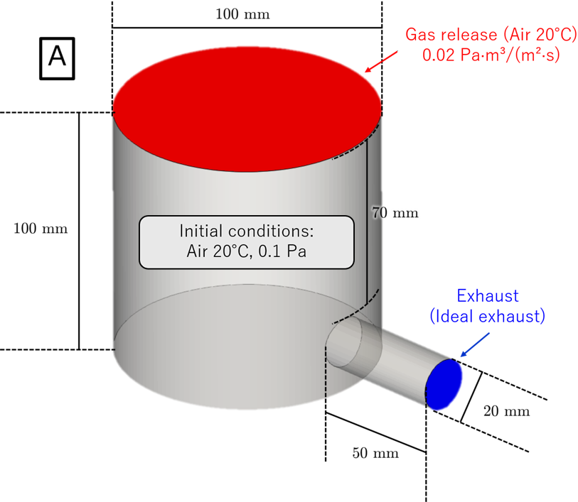
▲ Standard model (standard/A).
Consider a cylindrical vacuum chamber with a diameter of $100\ \mathrm{mm}$ and a height of $100\ \mathrm{mm}$,
to which a short cylindrical pipe with a diameter of $20\ \mathrm{mm}$ and a length of $50\ \mathrm{mm}$ is connected.
Assume that the end of the pipe (the blue surface in the figure) is ideally evacuated by a vacuum pump
(i.e., all gas molecules that reach it are removed)*1.
We also consider a case where there is a steady-state gas influx into the vacuum chamber,
assuming that air at $20^{\circ}\!\mathrm{C}$ enters the chamber predominantly
at a rate of $0.02\ \mathrm{Pa\cdot m^{3}/(m^{2}\cdot s)}$
at the top of the vacuum chamber (red surface in the figure).
As other conditions, the wall temperature of the vacuum chamber and piping is set to $20^{\circ}\!\mathrm{C}$,
and the initial conditions for the simulation (initial exhaust pressure) are
set to $0.1\ \mathrm{Pa}$ for air at $20^{\circ}\!\mathrm{C}$*2.
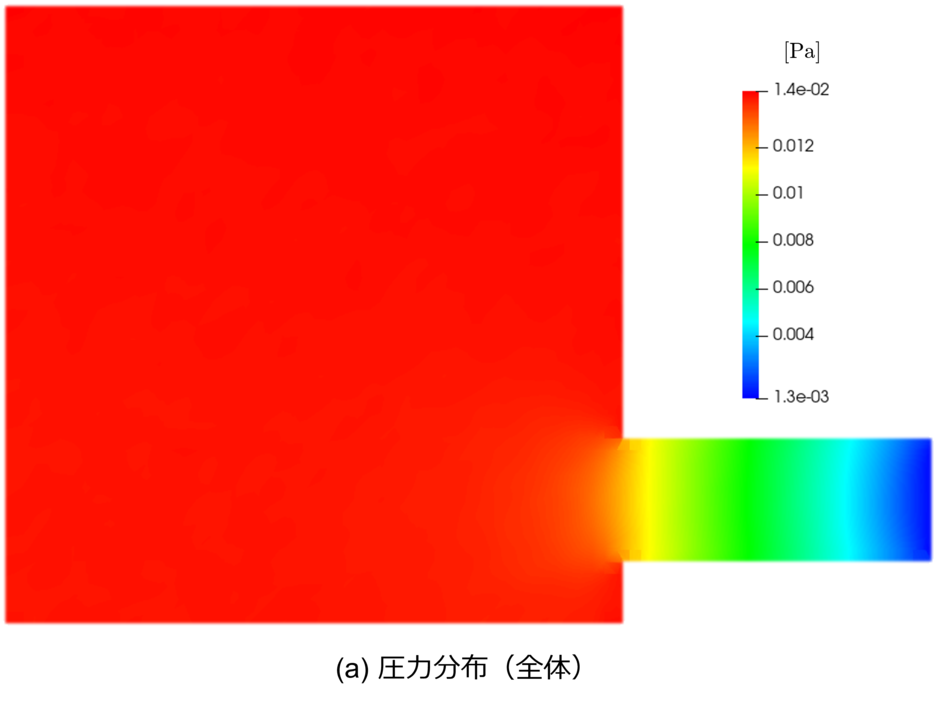
Exhaust simulations conducted under the above conditions yielded the results shown in the figure below.
 |
 |
 |
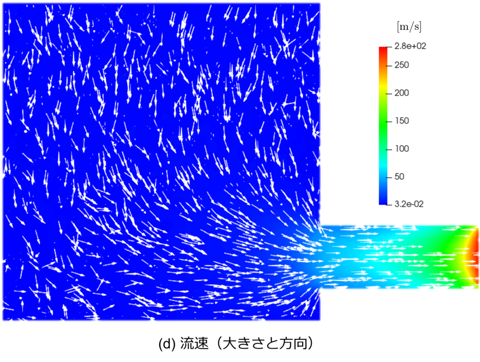 |
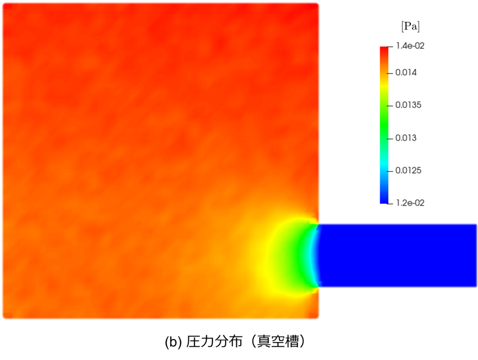
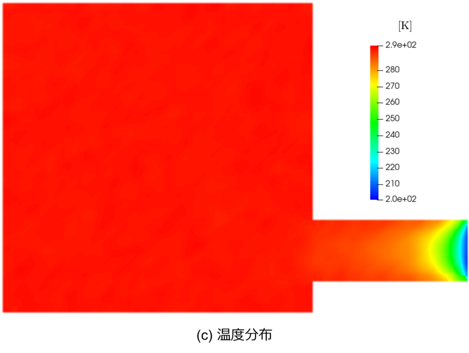
▲ Exhaust simulation results for the standard model (standard/A) (cross-sectional view). (a) Pressure distribution, (b) Pressure distribution within the vacuum chamber, (c) Temperature distribution, (d) Flow velocity (contours indicate magnitude; white arrows indicate direction).
It can be seen that the pressure inside the pipe decreases linearly from the inlet to the exhaust port.
Although the pressure inside the vacuum chamber remains nearly constant, strictly speaking,
there is a variation of ${+1.5\%}/{-15\%}$ in the average pressure within the chamber.
With the exception of the exhaust port, the temperature remains nearly constant at $20^{\circ}\!\mathrm{C}$.
In this case, we are assuming ideal exhaust conditions,
so the temperature decreases near the exhaust port because the molecular velocities become uniform (the dispersion decreases).
The velocity distribution also suggests that the velocities are uniform near the exhaust port.
Now, let’s use the simulation results to evaluate the conductance $C$ of the short cylindrical pipe.
Let $p_{\mathrm{in}}$ be the pressure at the pipe inlet, $p_{\mathrm{out}}$ be the pressure at the outlet, and $S$ be the pumping speed.
Since the pipe’s conductance can be calculated using
\begin{align*}
C = \frac{Sp_{\mathrm{out}}}{p_{\mathrm{in}}-p_{\mathrm{out}}},
\end{align*}
we can determine from the simulation results that the conductance of the short cylindrical pipe in standard/A is
\begin{align*}
C \sim 0.0120\ \mathrm{m^{3}/s}.
\end{align*}
On the other hand, the formula for the conductance $C_{\mathrm{f}}$ (where the subscript $\mathrm{f}$ stands for formulated) in the case of molecular flow is known for several cases;
for example [1], the conductance of a short cylindrical pipe for air at $20^{\circ}\!\mathrm{C}$ is given by
\begin{align*}
C_{\mathrm{f}} = K_{\mathrm{c}} \times 116A^{*3},
\end{align*}
where $K_{\mathrm{c}}$ is called the Clausing's factor, a quantity determined by the ratio $l/d$ of the pipe's diameter $d$ to its length $l$.
Furthermore, $A$ is the cross-sectional area of the pipe $\mathrm{(m^{3})}$.
If $l/d=2.5$ and $K_{\mathrm{c}}=0.318$, then
\begin{align*}
C_{\mathrm{f}} \sim 0.0116\ \mathrm{m^{3}/s}.
\end{align*}
There is a difference of $3.6\%$ relative to the theoretical value and $0.00041\ \mathrm{m^{3}/s}$ in absolute terms between the conductance $C$
obtained from the simulation and the conductance $C_{\mathrm{f}}$ obtained from the theoretical equation.
This is presumed to be a systematic discrepancy resulting from factors such as the theoretical equation not accounting for temperature distribution
within the piping and the pressure inside the vacuum chamber not being ideally uniform (the conductance of the vacuum chamber itself cannot be ignored).
Next, let's consider the pumping speed.
The effective pumping speed $S_{\mathrm{e}}$ (where the subscript $\mathrm{e}$ stands for effective)
of the piping and vacuum pump installed in the vacuum chamber can be expressed as
\begin{align*}
S_{\mathrm{e}} = \frac{SC}{S+C}.
\end{align*}
Therefore, the effective pumping speed obtained from the simulation (alone) is
\begin{align*}
S_{\mathrm{e}} = 0.0105\ \mathrm{m^{3}/s}.
\end{align*}
On the other hand, using the conductance calculated from the theoretical equation, we obtain
\begin{align*}
S_{\mathrm{e}}^{\prime} = \frac{SC_{\mathrm{f}}}{S+C_{\mathrm{f}}} \sim 0.0101\ \mathrm{m^{3}/s}.
\end{align*}
Due to the difference in conductance used to evaluate the effective pumping speed,
there is a relative difference of $3.1\%$ and an absolute difference of $0.00032\ \mathrm{m^{3}/s}$
between $S_{\mathrm{e}}$ and $S_{\mathrm{e}}^{\prime}$.
Now that we have determined the effective pumping speed, let's plot the pumping curve.
Let $p$ denote the pressure inside the vacuum chamber, $V$ denote its volume, and $Q$ denote the gas flow rate into the chamber.
The exhaust equation is then
\begin{align*}
V\frac{\mathrm{d}p}{\mathrm{d}t} = -S_{\mathrm{e}}p + Q.
\end{align*}
When the initial pressure is $p_{0}$, the solution to this differential equation is
\begin{align*}
p(t) = \left( p_{0} - \frac{Q}{S_{\mathrm{e}}} \right) \exp \left( -\frac{S_{\mathrm{e}}}{V} t \right) + \frac{Q}{S_{\mathrm{e}}}.
\end{align*}
This equation corresponds to the ideal pumping curve.
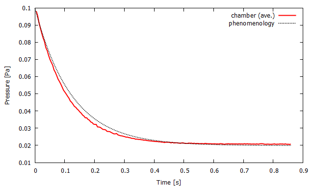
The figure below plots the time variation of the average pressure inside the vacuum chamber and the inlet pressure of the piping,
as determined by simulation, alongside the pumping curve derived phenomenologically using $S_{\mathrm{e}}$ as the effective pumping speed
and the pumping curve derived theoretically using $S_{\mathrm{e}}^{\prime}$.
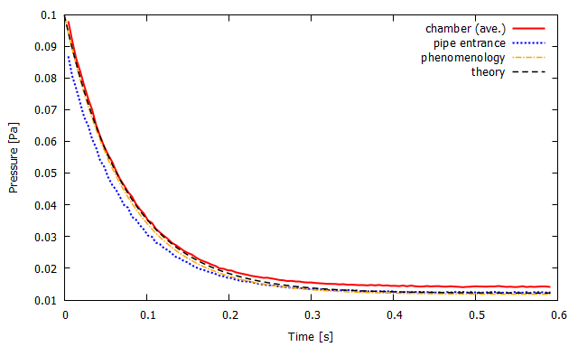
▲ Time-dependent changes in the average pressure inside the vacuum chamber (solid red line) and the pressure at the inlet of the piping (dashed blue line), along with the phenomenological pumping curve (dashed orange line) and the theoretical pumping curve (dashed black line).
The average pressure inside the vacuum chamber decreases almost ideally for a short time after the start of evacuation, but the evacuation efficiency gradually deteriorates, and the reach pressure reached is higher than the ideal value $Q/S_{\mathrm{e}}^{\prime}$. This is believed to be caused by factors such as the conductance of the vacuum chamber itself, as mentioned earlier, making evacuation more difficult than the theoretical value (i.e., the theoretical conductance value evaluated for the upper section is too high compared to the conductance of the entire system). On the other hand, it can be seen that the actual pressure reached at the pipe inlet matches the ultimate pressure $Q/S_{\mathrm{e}}^{\prime}$ - calculated based on the theoretically derived pipe conductance value - with high precision.
*1 To make the comparison with the theoretical equation easier to understand, we have assumed ideal exhaust conditions; however, in DSMC-Neutrals, it is also possible to specify the pumping speed and pressure as outflow boundary conditions.
*2 Since the Knudsen number for air at $20^{\circ}\!\mathrm{C}$ is approximately $K_{\mathrm{n}}=6.6/(pL)$ (where $p$ is pressure $\mathrm{(Pa)}$ and $L$ is the characteristic length $\mathrm{(mm)}$), applying this to standard/A yields $K_{\mathrm{n}}\gt 1$ for both the vacuum chamber and the piping; therefore, molecular flow behavior is expected. Since we will later compare the results with theoretical equations, the equations become complex in the viscous flow regime. Therefore, for the sake of simplicity, we will examine exhaust from the initial pressure in the molecular flow regime in this study; however, it is also possible to perform exhaust simulations starting from higher pressures using DSMC-Neutrals.
*3 This equation uses the conductance of a theoretically derived (thickness-independent) orifice as a reference and reduces the effect of thickness to Clausing's factor. For convenience, we will refer to this equation as the "theoretical equation".
[1] S. Dashman, "Scientific foundation of vacuum technique", New York, John Wiley & Sons (1949).
Pipe Connected in Series and Parallel
Next, let’s compare the results for the cases where the exhaust pipes are connected in series (simulation model long/B) and in parallel (simulation model parallel/C), as shown in the figure below, with the results from the previous simulation model standard/A.
 |
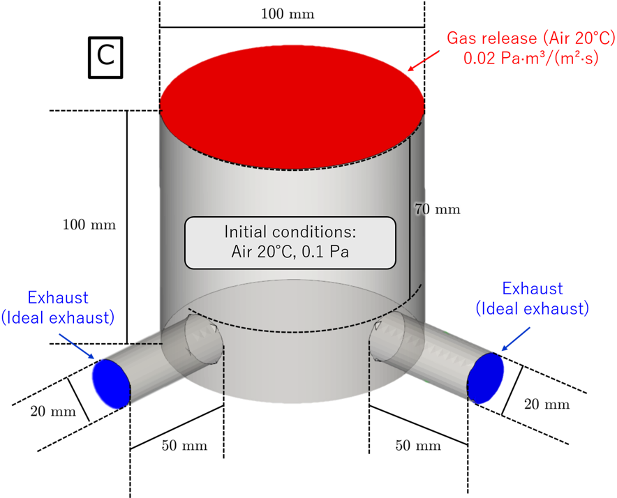 |
▲ Pipe series connection model (long/B) and pipe parallel connection model (parallel/C).
The graph below shows the average pressure inside the vacuum chamber, as tracked by the simulation, plotted for each of the simulation models A, B, and C.
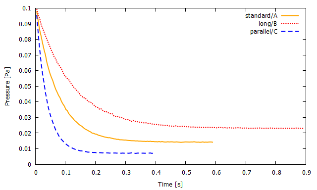
▲ Average pressure inside the vacuum chamber for standard/A (solid orange line), long/B (red dotted line), and parallel/C (blue dashed line).
The equivalent conductance of pipes connected in series is the reciprocal of the sum of the reciprocals of their individual conductances;
thus, the equivalent conductance of pipes with the same conductance $C$ connected in series is approximately $(1/2)C$.
On the other hand, the equivalent conductance when pipes are connected in parallel is the simple sum of their individual conductances;
therefore, if pipes with the same conductance $C$ are connected in parallel, the equivalent conductance is $2C$.
Looking at the graph, we can see that lower reach pressures are indeed achieved in order of increasing conductance (i.e., pipes through which gas flows more easily).
Next, let's focus on models B and C and compare the simulation results with the theoretically derived conductance and effective pumping speed.
Here, please note an important point regarding the theoretical derivation of conductance: in this case,
long/B should not be treated as the combined conductance of two short cylindrical pipes, each $50\ \mathrm{mm}$ long,
but rather as the conductance of a single short cylindrical pipe $100\ \mathrm{mm}$ long.
(For a rough calculation where precision is not critical, an estimate of the combined conductance, as in the comparison above, is acceptable.)
Now, let’s compare the conductance $C$evaluated by simulation and the conductance $C_{\mathrm{f}}$ calculated from the theoretical equation *4
with the corresponding actual exhaust velocities $S_{\mathrm{e}}$ and $S_{\mathrm{e}}^{\prime}$.
First, summarizing the results for long/B:
\begin{align*}
C_{\mathrm{(B)}} &\sim 0.00624\ \mathrm{m^{3}/s},&
\quad
C_{\mathrm{f(B)}} &\sim 0.00725\ \mathrm{m^{3}/s},
\\
S_{e\mathrm{(B)}} &\sim 0.00577\ \mathrm{m^{3}/s},&
\quad
S_{\mathrm{e(B)}}^{\prime} &\sim 0.00662\ \mathrm{m^{3}/s}.
\end{align*}
The difference in conductance was $14\%$ relative and $0.0010\ \mathrm{m^{3}/s}$ absolute.
The difference in effective pumping speed was $13\%$ relative and $0.00086\ \mathrm{m^{3}/s}$ absolute.
Next, summarizing the results for parallel/C:
\begin{align*}
C_{\mathrm{(C)}} &\sim 0.0241\ \mathrm{m^{3}/s},&
\quad
C_{\mathrm{f(C)}} &\sim 0.0232\ \mathrm{m^{3}/s},
\\
S_{e\mathrm{(C)}} &\sim 0.0208\ \mathrm{m^{3}/s},&
\quad
S_{\mathrm{e(C)}}^{\prime} &\sim 0.0203\ \mathrm{m^{3}/s}.
\end{align*}
The difference in conductance was $3.9\%$ relative and $0.00090\ \mathrm{m^{3}/s}$ absolute.
The difference in effective pumping speed was $2.2\%$ relative and $0.00046\ \mathrm{m^{3}/s}$ absolute.
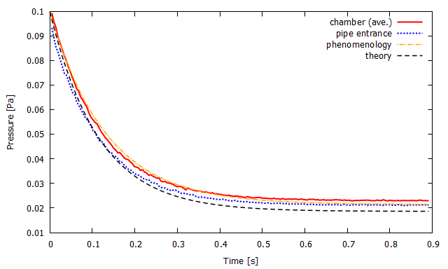
The graph below shows the time-dependent changes in the average pressure inside the vacuum chamber and the inlet pressure of the piping,
as tracked by simulation for Models B and C, plotted alongside phenomenological and theoretical pumping curves.
 |
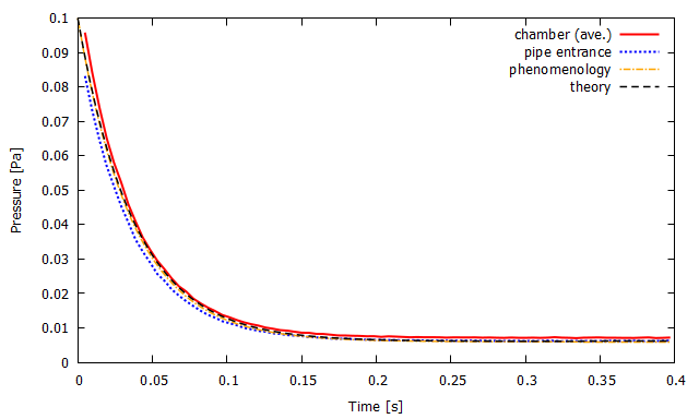 |
▲ Time-dependent changes in the average pressure inside the vacuum chamber (solid red line) and the pressure at the inlet of the piping (dashed blue line), along with the phenomenological pumping curve (orange dotted line) and the theoretical pumping curve (black dashed line). (Left) long/B. (Right) parallel/C.
Calculation long/B shows that the actual exhaust performance is worse than the theoretical value.
We will discuss this later.
In contrast, parallel/C agrees well with the theoretical values.
As with standard/A, the agreement is such that the average pressure inside the vacuum chamber is initially evacuated ideally,
and the pressure at the pipe inlet eventually matches the theoretical ultimate pressure almost exactly.
*4 For a short cylindrical pipe $100\ \mathrm{mm}$ long and $20\ \mathrm{mm}$ in diameter, the Clausing's factor was set to $K_{\mathrm{c}}=0.199$. Also, for reference, when calculating the combined conductance of two $50\ \mathrm{mm}$ short cylindrical pipes, \begin{align*} C_{\mathrm{f}(100\ \mathrm{mm})} \simeq \frac{1}{2\times\frac{1}{C_{\mathrm{f}(50\ \mathrm{mm})}}} \sim 0.00579\ \mathrm{m^{3}/s}. \end{align*}
Effect of Orifice in Pipe
Next, let’s examine the case where an orifice is installed in the exhaust pipe, as shown in the figure below. In this section, we will consider two simulation models: one with an orifice inner diameter of $10\ \mathrm{mm}$ (simulation model orifice (10 mm)/D) and another with an inner diameter of $15\ \mathrm{mm}$ (simulation model orifice (15 mm)/E).
 |
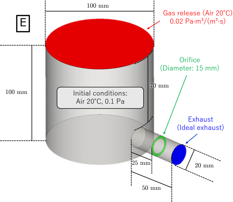 |
▲ Models with an orifice inner diameter of $10\ \mathrm{mm}$ (orifice (10 mm)/D) and $15\ \mathrm{mm}$ (orifice (15 mm)/E).
First, let's compare the time variation of the average pressure inside the vacuum chamber with that of the standard/A.
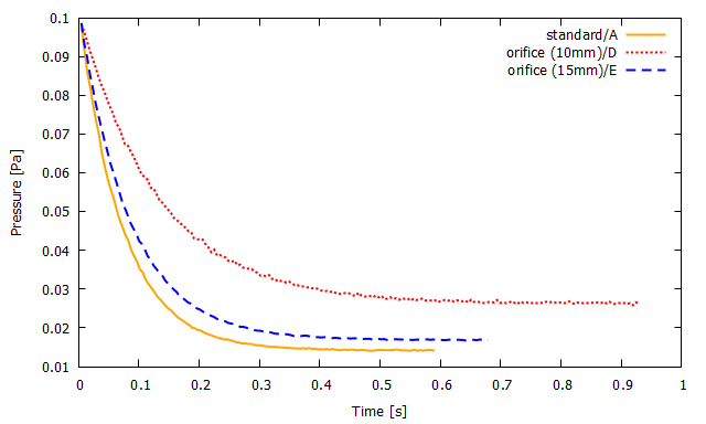
▲ Average pressure inside the vacuum chamber for standard/A (solid orange line), orifice (10 mm)/D (red dotted line), and orifice (15 mm)/E (blue dashed line).
While it is self-evident that as the orifice diameter decreases, the conductance decreases and the pressure at the outlet increases,
we were able to obtain specific pumping curves through simulation.
Now, as we have done previously, let’s compare the conductance $C$ evaluated by simulation and the conductance $C_{\mathrm{f}}$ calculated from the theoretical equation*4
with the corresponding actual exhaust velocities $S_{\mathrm{e}}$ and $S_{\mathrm{e}}^{\prime}$.
Here, as shown in [2], it is known that the conductance of an orifice in a pipe can be expressed as
\begin{align*}
C_{\mathrm{f(orifice\ in\ pipe)}} = K\frac{116A}{1-A/A_{0}},
\end{align*}
where $A$ represents the cross-sectional area of the orifice $\mathrm{(m^{2})}$,
and $A_{0}$ represents the cross-sectional area of the pipe $\mathrm{(m^{2})}$.
Furthermore, $K$is a correction factor similar to the Clausing's factor mentioned above, and its value is determined by the ratio of the pipe’s inner diameter to the orifice’s inner diameter.
To summarize the results for orifice (10 mm)/D*5:
\begin{align*}
C_{\mathrm{(D)}} &\sim 0.00560\ \mathrm{m^{3}/s},&
\quad
C_{\mathrm{f(D)}} &\sim 0.00607\ \mathrm{m^{3}/s},
\\
S_{e\mathrm{(D)}} &\sim 0.00524\ \mathrm{m^{3}/s},&
\quad
S_{\mathrm{e(D)}}^{\prime} &\sim 0.00565\ \mathrm{m^{3}/s}.
\end{align*}
The difference in conductance was $7.8\%$ relative and $0.00047\ \mathrm{m^{3}/s}$ absolute.
The difference in effective pumping speed was $7.3\%$ relative and $0.00041\ \mathrm{m^{3}/s}$ absolute.
Next, summarizing the results for orifice (15 mm)/E*6:
\begin{align*}
C_{\mathrm{(E)}} &\sim 0.00954\ \mathrm{m^{3}/s},&
\quad
C_{\mathrm{f(E)}} &\sim 0.00950\ \mathrm{m^{3}/s},
\\
S_{e\mathrm{(E)}} &\sim 0.00854\ \mathrm{m^{3}/s},&
\quad
S_{\mathrm{e(E)}}^{\prime} &\sim 0.00851\ \mathrm{m^{3}/s}.
\end{align*}
The difference in conductance was $0.36\%$ relative and $0.000034\ \mathrm{m^{3}/s}$ absolute.
The difference in effective pumping speed was $0.32\%$ relative and $0.000027\ \mathrm{m^{3}/s}$ absolute.
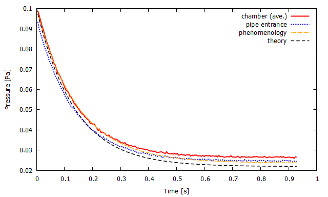
The graph below shows the time-dependent changes in the average pressure inside the vacuum chamber and the inlet pressure of the piping,
as tracked by simulation for Models D and E, plotted alongside phenomenological and theoretical pumping curves.
 |
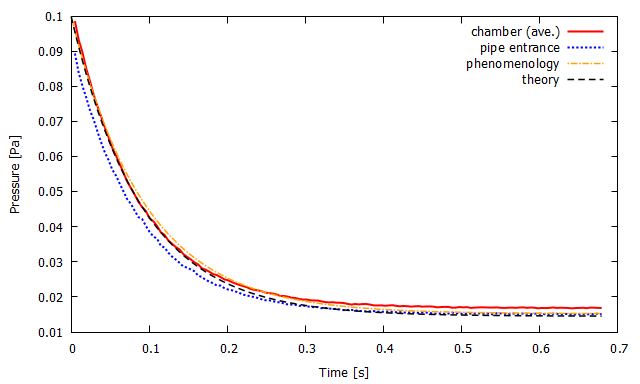 |
▲ Time-dependent changes in the average pressure inside the vacuum chamber (solid red line) and the pressure at the pipe inlet (dashed blue line), along with the phenomenological pumping curve (orange dotted line) and the theoretical pumping curve (black dashed line). (Left) model orifice (10 mm)/D. (Right) model orifice (15 mm)/E.
As with long/B, orifice (10 mm)/D shows that the actual exhaust performance is worse than the theoretical value.
We will discuss this later, along with long/B.
In contrast, orifice (15 mm)/E agrees well with the theoretical values, just as parallel/C does.
Initially, the average pressure inside the vacuum chamber is ideally evacuated, and ultimately,
the pressure at the inlet of the piping matches the theoretical ultimate pressure almost exactly.
*5 The correction factor was set to $K\simeq 1.049$.
*6 The correction factor was set to $K\simeq 1.127$.
[2] 熊谷寛夫,富永五郎,『真空の物理と応用』,裳華房 (1970).
Effect of Baffle
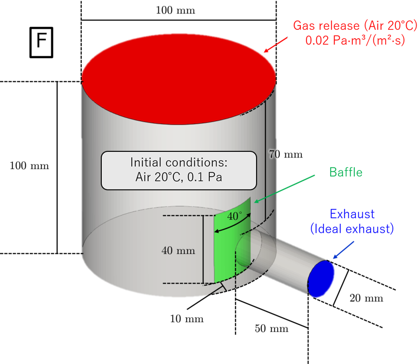
Finally, we will perform an exhaust simulation based on the scenario shown in the figure below, where a baffle is used to prevent contamination of the piping. In this simulation, we will consider two scenarios: one where the baffle is positioned $10\ \mathrm{mm}$ from the piping (simulation model “baffle/F”) and another where it is positioned $5\ \mathrm{mm}$ from the piping (simulation model “closer baffle/G”).
 |
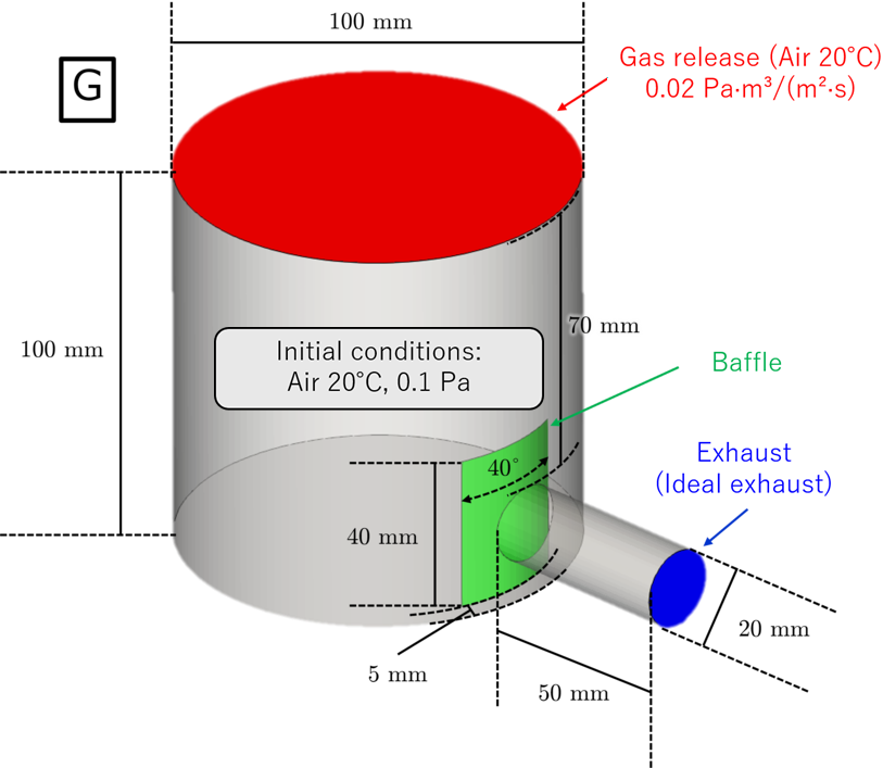 |
▲ Two models with different baffle configurations (baffle/F and closer baffle/G).
In this section, let’s compare the time evolution of the pressure at the center of the vacuum chamber with that of simulation model standard/A.
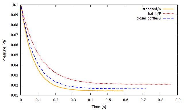
▲ Average pressure inside the vacuum chamber for standard/A (solid orange line), orifice (15 mm)/E (red dotted line), and closer baffle/G (blue dashed line).
One might expect that the narrower the flow path leading to the pipe inlet, the lower the conductance;
indeed, the graph confirms this result.
Since there is (probably) no known theoretical expression for the conductance of such models,
it is typically evaluated using Monte Carlo simulations.
By using DSMC-Neutrals, it is possible to simulate and evaluate the conductance of vacuum devices of any shape.
The conductance and effective pumping speed (of the piping and baffle section) evaluated through simulation were
\begin{align*}
C_{\mathrm{(F)}} \sim 0.00880\ \mathrm{m^{3}/s},
\quad
S_{e\mathrm{(F)}} \sim 0.00794\ \mathrm{m^{3}/s}
\end{align*}
for orifice (15 mm)/E,
\begin{align*}
C_{\mathrm{(G)}} \sim 0.00672\ \mathrm{m^{3}/s},
\quad
S_{e\mathrm{(G)}} \sim 0.00621\ \mathrm{m^{3}/s}
\end{align*}
for closer baffle/G.
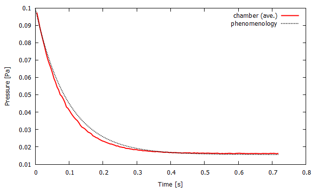
For Models F and G, respectively, the graph below was obtained by plotting the average pressure inside the vacuum chamber,
as tracked by simulation, alongside the phenomenological pumping curve.
 |
 |
▲ Time evolution of the average pressure inside the vacuum chamber (solid red line) and the phenomenological pumping curve (dashed black line). (Left) baffle/F. (Right) closer baffle/G.
The discrepancy between the average pressure inside the vacuum chamber and the pumping curve in the raw simulation data is believed to stem from uncertainties in the estimation of the chamber’s volume, which are caused by factors such as pressure distribution within the chamber.
Consideration and Summary
So far, we have compared the simulation results with theoretical conductance values and pumping curves.
While we have confirmed that the overall trends of the two are consistent, discrepancies from the theoretical curves were observed in models B and D.
Finally, let’s examine these discrepancies.
For now, we will express the difference between the theoretical conductance value $C_{\mathrm{f}}$ and the simulation result $C$ as $\Delta C$, i.e.,
\begin{align*}
C_{\mathrm{f}} = C + \Delta C,\quad \text{or} \quad \Delta C = C_{\mathrm{f}} - C.
\end{align*}
In this case, the relationship between the theoretical value $C$ and the difference $\Delta C$ is shown in the graph below.
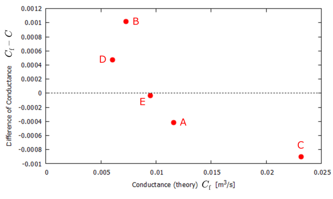
▲ Differences between simulation results and theoretical values for conductance.
Looking at the graph, it appears there may be a negative correlation between $C$ and $\Delta C$, but with so few data points, this is not certain.
However, at least as far as the magnitude of the difference $|\Delta C|$ is concerned,
it seems unlikely that it would be of an extremely large order (greater than $O(10^{-3})$) within the current data range).
(It is unlikely that the relative difference between the theoretical value and the simulation results would suddenly jump to $50\%$ or $100\%$ or more.)
On the other hand, let us consider the ultimate pressure $P_{\mathrm{u}}$ (the pressure at time $t\to\infty$),
which is a key value in the pumping curve.
Since there is also a discrepancy between the simulation results and the theoretical value for the peak pressure, we can express this as
\begin{align*}
\Delta P_{\mathrm{u}} = P_{\mathrm{u}}^{\prime} - P_{\mathrm{u}}
= \frac{Q}{S_{\mathrm{e}}^{\prime}} - \frac{Q}{S_{\mathrm{e}}}.
\end{align*}
Now, from the law of error propagation, we have
\begin{align*}
\left(\Delta P_{\mathrm{u}}\right)^{2}
= \left(\frac{\partial P_{\mathrm{u}}}{\partial C}\right)^{2} \left(\Delta C\right)^{2}
= \left(\frac{\partial}{\partial C}\frac{Q}{S_{\mathrm{e}}}\right)^{2}\left(\Delta C\right)^{2}
= \left(\frac{\partial}{\partial C}\frac{Q(S+C)}{SC}\right)^{2}\left(\Delta C\right)^{2}
= \left(\frac{Q}{C^{2}}\right)^{2}\left(\Delta C\right)^{2},
\quad
\text{i.e.}\quad \left|\Delta P_{\mathrm{u}}\right| = \left|\frac{Q}{C^{2}}\Delta C\right|.
\end{align*}
This equation implies that, unless the rate of change of $\Delta C$ exceeds the rate of change of $C^{2}$,
the smaller the conductance value $C$,
the larger the difference $\Delta P_{\mathrm{u}}$ between the simulated and theoretical values of the ultimate pressure.
In fact, plotting the theoretical conductance value $C$ against the pressure difference $\Delta P_{\mathrm{u}}$ yields the graph shown below.
This provides a qualitative explanation for why the simulation results differ significantly from the theoretical pumping curves in models B and D,
while they agree quite well in the other models.
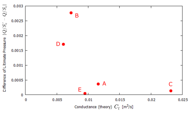
▲ Differences between simulation results and theoretical values regarding the pressure at the outlet.
As described above, performing simulations using DSMC-Neutrals allows us to investigate aspects that cannot be determined through theoretical analysis alone,
as well as the differences between the ideal conditions assumed by theory and actual devices.
Furthermore, it is possible to evaluate the conductance of complex devices,
such as vacuum systems equipped with baffles, for which theoretical estimates cannot be made.
We hope this column has sparked your interest in exhaust simulations.
If you have any questions or concerns, please don’t hesitate to contact us!